Is There a Trend in Global Average Temperature?

John Reid

Introduction

This article is intended as a popular account of my paper in Energy and Environment (Reid 2017) which recently appeared on-line. It includes no equations or mathematical symbols.

But what about the volcanoes?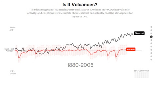

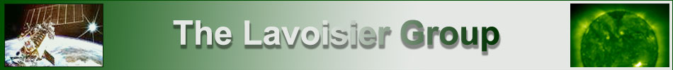
Figure 1: Image from the Bloomberg Web site demonstrating that global temperature change is not
due to sub-aerial volcanoes.

In June 2015 in an online article in Bloomberg entitled "What is Really Warming the World" graphs were presented demonstrating that increases in global average temperature since 1880 are due neither to orbital changes, changes in solar activity, volcanic activity, deforestation, ozone changes nor sulphate aerosols. Figure 1 is a reproduction of one of these graphs. Only atmospheric CO2 concentrations resemble the observed increase. Unsurprisingly they conclude that increases in greenhouse gases must be causing the observed temperature changes.

Unfortunately the authors seem unaware of the simplest and most obvious correlation, i.e. the correlation of global average temperature with its value in each preceding year. Figure 2 demonstrates this graphically.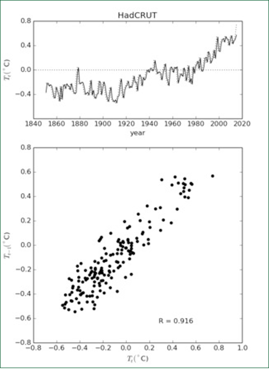

Figure 2: Top: HadCRUT global average temperature (solid line) and previous year's global average temperature (dotted line). Bottom: Scatter diagram of global average temperature vs previous year's global average temperature. The sample correlation coefficient is 0.916.

The correlation between temperature values in successive years is 91.6%. This may seem trivial and unimportant, but it is not. It reveals that the temperature time series is either a "random walk" or is close to being a random walk, that it has a "pole near zero frequency". It shows that a large fraction of the total variance is associated with low frequencies and long time scales and that we must be therefore be very cautious about assuming overly simplistic causes for the observed variations.

These ideas are well understood by researchers versed in signal processing theory or Econometrics but not, it appears, those working in climate science. In order to understand this more fully we need to first understand the difference between "deterministic" and "stochastic" world views.

Deterministic vs Stochastic

There are two views of the natural world. Either

a) it is deterministic meaning that the future is completely determined by the present or

b) it is stochastic meaning that future is not completely determined by the present but contains an additional, unknown, random component.

The word "stochastic" means "governed by the laws of probability".

All the variables in every state of a deterministic system can be expressed as functions of time as if the system under investigation were a machine. Such a mechanistic description allows the precise prediction the state of the system at any future time. The only practical limitations are presumed to be the computer word length and the measurement error of real-world observations against which the model predictions are to be tested. The reliability of the predictions of a fully deterministic model do not decrease in precision with time.

Stochastic variables can only be mathematically expressed as functions, not of time, but of past states. They include an additional, unselfcorrelated, random component known as "the innovation". As a consequence when we use a stochastic model to predict further and further into the future, the predictions become less and less reliable because randomness accumulates from one predicted state to the next. This leads to the idea of a "prediction horizon" as described by Koutsoyiannis (2010), for example, the weather has a prediction horizon of about a week.

Stochastic models have a built-in, self-testing mechanism. When a stochastic model is proposed, the innovations can be estimated from the data. These estimates are termed "residuals". The residuals are tested and if they are self-correlated, the model must be rejected. In this way stochastic models enable the rigorous testing of models against data in accordance with the scientific method as described, for example, by Popper (1963). Intuitively speaking, any self-correlation implies that some information about the system remains behind in the residuals and has not been properly accounted for by the model being tested. There are well-established statistical tests for evaluating stochastic models in this way. Note that it is the model itself which is being tested; providing confidence limits for the values of model parameters is a different process.

It might be argued that deterministic numerical models (i.e. computer models) are more closely related to the underlying physics than are stochastic models but that is not necessarily the case. In practice numerical models are often unstable and "blow-up" or "go to infinity" when certain conditions are not met. Modellers then fix the problem by smoothing the boundary conditions and/or arbitrarily increasing frictional terms in order to keep the model stable. Needless to say, the physics of the model soon ceases to resemble the physics of the real world.

Perhaps the worst aspect of the deterministic world-view is the mechanistic head-set that goes with it, i.e. the belief that the natural world is a clockwork mechanism in which every quantity can ultimately be expressed as an explicit function of time. This leads to a pointless search for "trends", "cycles" and "oscillations" in real world data. The reality of such trends and cycles is never doubted by their proponents. The deterministic assumption precludes any objective basis for statistical inference.

A stochastic model may, of course, contain deterministic components in the form of trends and periodic cycles along with stochastic components. The presence or absence of such deterministic elements can be tested by the usual statistical methodology, viz.: by computing the probability that a possible trend or cycle in the data could have occurred purely by chance and, should this probability be less than some agreed threshold, then the trend or cycle is regarded as real.

A powerful concept to come out of the stochastic approach is that of the "random walk". A random walk occurs when random quantities are accumulated in a running total. For example if we toss a coin many times and subtract the number of tails from the number of heads, the cumulative difference is a random walk. On average the proportion of heads approaches fifty per cent, but the magnitude of the difference between the number of heads and the number of tails increases indefinitely. The difference is a random walk.

A physical example of a random walk are temperature measurements of a pond taken at regular intervals as random amounts of heat are added or subtracted from the pond between one measurement and the next by natural processes. However unlike the coin toss example there are limits to the extent of the temperature variation. If the pond gets very cold during a cold spell it will absorb heat faster on a typical day. Likewise when it gets warmer it will cool faster on a typical day. This is called a "centrally biased random walk". It is easier to consider because it is statistically well behaved (i.e. stationary); the pond temperature does not increase or decrease indefinitely.

Over short time intervals random walks often exhibit apparent trends and cycles. Two unrelated random walk quantities may appear to be correlated with one another even though they are truly independent. The way in which a gambler's accumulated capital rises and falls according to his wins and losses in a fair casino is another example of a random walk. It will exhibit an upward trend when the gambler has a "run of luck". As gamblers are aware, such upward trends are rarely sustained, particularly in real casinos. They are spurious trends.

Random walks are not "nice" statistically; they exhibit spurious correlations and false trends.

This was first noted by George Udny Yule in his 1926 Presidential Address to the Royal Statistical Society. More recently Granger and Newbold (1974) pointed out the dangers of what they called "spurious regression" in econometric time series. A decade later Nelson and Kang (1984) realized that spurious trends are sometimes seen when data are regressed on time as the independent variable, i.e. when a straight line is fitted to the data with time plotted along the horizontal axis. These problems occur when the data is a random walk or a centrally biased random walk. In signal processing terms, they occur when the data has a "red" spectrum, i.e. when the bulk of the variance occurs at low frequencies. Apart from Econometrics there has been little discussion of spurious regression in other areas of research.

Application to Global Average Temperature

Figure 3a shows the HadCRUT time series of global average temperature. If we assume that this time series has been deterministically generated, we can plot a linear trend as shown by the solid line. Better still we can add a sinusoidal curve to the linear trend and make the fit even better.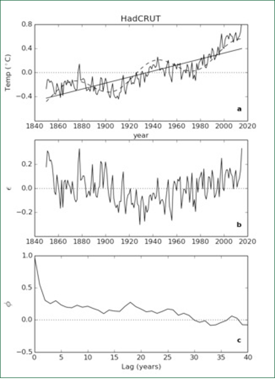

Figure 3: (a) HadCRUT time series of global average temperature 1850 - 2015 showing a linear "trend" (solid line) and a trend plus a multidecadal "cycle" (dashed curve). (b) Residuals remaining after subtracting the dashed curve from the original data. (c) Autocorrelation of the residuals.

When the linear trend plus curve values are subtracted from the original data we get the time series of residuals shown in Figure 3b. The sample autocorrelation function of the residuals is shown in Figure 3c. Both Figures 3b and 3c indicate that there is still some fitting left to be done. We can go on adding sinusoids until we get a fit as good as we wish as we all know from Fourier's Theorem.

This process is called "curve fitting". Curve fitting can be done with sinusoids, with wavelets, with Legendre polynomials or with any orthogonal set of functions and can give spectacular results for display purposes. The problem with such curve fitting exercises is that they tell us very little about underlying processes and, worse still, tend to fail dramatically outside the range of the fit. They have little or no predictive power. Assuming that a deterministic mechanism underpinned the data allowed us to fit the curve but it told us nothing about the nature of the mechanism.

Instead suppose we make the alternative assumption that the data is the outcome of a stochastic process. Using standard statistical package we can fit a model known as an "Autoregressive Moving Average" (ARMA) model to the data. Furthermore, under this stochastic assumption, the presence or absence of a linear trend (such as that depicted by the solid line in Figure 3a), can be independently tested. It is known as a "drift term" because, if it is real, it means there is a systematic drift between one value of temperature and the next.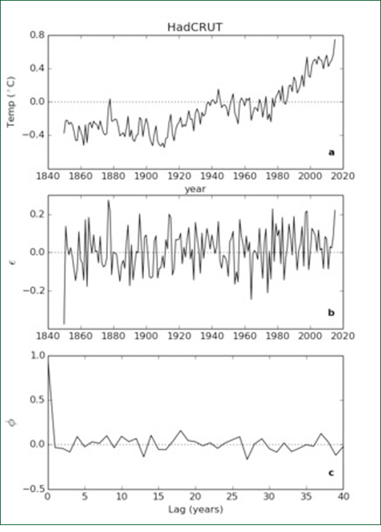

Figure 4: (a) The HadCRUT time series shown in Figure 3a. (b) Time series of residuals after fitting an ARMA(1,2) model to the data. (c) Autocorrelation function of the residuals.

An ARMA (1,2) model with a drift term was found to fit the HadCRUT time series, which means that one autoregression coefficient and two moving average coefficients were needed. The residuals from the model fit are shown in Figure 4b and their autocorrelation function in Figure 4c. This time the residuals look like white noise and this is confirmed by their autocorrelation function being close to zero at all non-zero lags. Even better, the residual correlations can be tested using two sophisticated tests, the Ljung-Box test and the Bruesch-Godfrey test. The sequence of residuals passed both tests indicating that the residual were unselfcorrelated implying, in turn, that the ARMA(1,2) model is an excellent fit to the data.

Most importantly, the drift term was found to be not significantly different from zero.

Intuitive explanations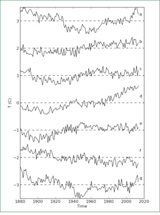

Figure 5: The original global average temperature time series together with six artificially generated time series each with the same statistical structure as the original series.. The reader is invited to decide which series is the odd one out.

An advantage of the stochastic ARMA description of a time series is that, once the ARMA coefficients are known it becomes possible to artificially generate time series which are statistically identical to the given time series but with a different innovation. The artificial time series is identical with the original in that it has the same population autocorrelation function and the same variance spectrum.

Six time series were generated in this way and are displayed alongside the original HadCRUT time series in Figure 5. It can be seen that all seven graphs have the same "look" or character; none stand out as being obviously different. (The original is, of course, 5d.) We can conclude that the 0.8°C observed increase in temperature between 1850 and 2015 is simply a consequence of the red, stochastic character of the time series; it does not have an immediate "cause". It is the consequence of myriads of energetic interactions in the terrestrial environment in which heat is gained and lost to and from the land and the oceans.

Likewise if we were to compute the sample correlation coefficient holding between (b) and (d), say, it would no doubt turn out to be significantly positive even though we know there is no connection between the two samples. The latter is an example of the "spurious regression" of Udny Yule and Granger and Newbold.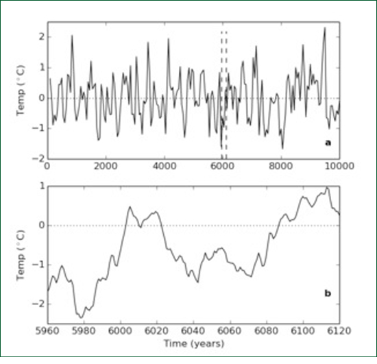

Figure 6: (a) A 10,000-long time series artificially generated using the parameters estimated from the original series. (b) A short, 160-long sub-sample of this series which resembles the observed series of global average temperatures.

A second intuitive explanation is illustrated by Figure 6. Figure 6a shows a time series 10,000 "years" long which was generated using the ARMA parameters estimated from the data. This is about the same length of time as the present Holocene epoch which followed the last Ice Age and indeed the series strongly resembles the time series of proxy temperature data for this period obtained from ice cores (without drift). It is immediately obvious that the series is stationary - it shows no tendency to trend toward plus or minus infinity. Secondly it looks a bit cyclic. This is an illusion. No cycles are actually present. What we are viewing is low-pass filtered white noise with a cut-off period of about a millennium. If we sample with a time interval greater than the cut-off it looks white. If the time period is shorter than a millennium it looks red. If we sample it annually for 160 years, the length of the HadCRUT sample, say from 5960 to 6120 (Figure 6b), to see the fine structure, we see something that exhibits an apparent rising trend plus a multi-decadal oscillation very much like the original HadCRUT time series.

In this case we are quite sure that neither the trend nor the oscillation are real. They are just red noise. Why should we believe that that the trend and oscillation exhibited by HadCRUT are real? Certainly we cannot prove that they are not real but then there is a well established principle called Occam's Razor which says that if you already have a satisfactory explanation for an observed phenomenon (i.e. that it is red noise) there is no point in adding extra theories. As Laplace said to Napoleon about God: "I have no need of that hypothesis"

A legal analogy

The argument put forward in the Bloomberg article associated with Figure 1 above was presented in a more rigorous form by Kokic et al (2014). These authors ran an ARMA model similar to the one discussed here but they also included a number of additional regression terms including solar radiation, volcanic forcing, and El Nino Southern Oscillation as well as atmospheric CO2 concentration. They found the regression coefficient of CO2 concentration to be significant. However they seem unaware of the possibility of spurious regression and the work of Granger and Newbold was not mentioned.

It appears then, that if we include a regression term in the model for CO2 it will show a significant relationship with temperature and, if we do not, everything is still okay? Maybe there is some spurious regression happening here, maybe not. What is going on? Consider a legal analogy. A crime has been committed: the increase in global average temperature. CO2 stands accused. There is evidence that CO2 is implicated.

But wait! Has a crime actually been committed? The non-significant drift coefficient of Reid (2017) implies that it has not. If there is no actually crime, there is no point in fitting up CO2 as the perpetrator however much we may dislike him.

Conclusion

There is no significant trend in global average temperature and therefore no need to look for causes. At time scales of less than a millennium global temperature variations are just red noise.

References

Granger, C.W.J. and P. Newbold (1974). Spurious regressions in Econometrics. J. Econometrics 2, 111-120.

Kokic, P., S. Crimp and M. Howden (2014). A probabilistic analysis of human influence on recent record global mean temperature changes. Climate Risk Management, 3, 1-12.

Koutsoyiannis, D. (2010). A random walk on water. Hydrol. Earth Syst. Sci., 14, 585-60.

Nelson C.R. and H. Kang (1984). Pitfalls in the use of time as an explanatory variable in regression.J. Business Econom Stat, 2 73-82.

Popper, K. (1963), Conjectures and Refutations, Routledge and Keagan Paul, London. See: http://www.scienceheresy.com/scienceheresyarchive/2010_10/Popper/index.html

Reid, J.S. (2017). There is no significant trend in global average temperature. Energy and Environment, 28, 3, 302-315.

Udny Yule, G. (1926). Why do we sometimes get nonsense correlations between time series? J. Roy. Stat. Soc., 89, 1-69.